Radio Physics for Wireless Devices and Networking

 

By Ron Vigneri Rev: 8-26-13 Update of 10-8-2008 Article

 

Note: This material is applicable to any electromagnetic wave (broadcast) technology

including:  Wi-Fi, radio, television, cellular telephone, radar, etc. Someone adding this

knowledge to his skill set is a good candidate for wireless computer networking,

cellular telephone, and/or related industries.

 

The Radio Physics of Wi-Fi

 

The standard for wireless LANs (WLANs) was completed in 1997 with the release

of the IEEE 802.11 specification which became the first major step in the development

of wireless network technologies. The spread of the technology is similar to

that of cellular telephone. Wireless technology is one the hottest items in

networking for the home, office, and even wide area (WAN) applications like

high speed Internet access. This is the case with the recent broadband

wireless deployments by AT&T, Verizon, Sprint, and others. Let’s see the physics

involved in everyday wireless technology in this lesson, which is updated to include the

latest 802.11ac pre-release specification.

 

Radio Wave Physics

 

A radio wave is an electromagnetic wave that can propagate (travel) through

air, water, walls, some objects, and the vacuum of outer space. The wave is

an electric field and an associated magnetic field at right angles

to each other. Both these fields can vary periodically in amplitude and frequency.

The fields vary perpendicularly to the direction of propagation of the radio

wave. The fields, and hence, the radio wave can be generated by applying an

alternating current (or voltage) to a dipole (two conductor) antenna. The frequency of the

alternating current for the exercises in our study will be considered to be 2.4 gigahertz

(2.4 GHz), which is an unlicensed frequency regulated by the FCC. In the present Wi-Fi

standards another unlicensed frequency for use is 5 GHz .

 

So, electromagnetic waves consist of the propagation of oscillating electric

and magnetic fields shown in the following diagram. Note that

as the radio wave propagates (radiates) out from the dipole antenna source we

considered. It will decrease in amplitude (the “height” of the fields in the

diagram) as it travels farther from the source due to loss factors.

 

 

 

Fig. 1 Electromagnetic Wave

 

In the above illustration, the frequency of the electromagnetic wave can be

determined from the time period (T). The time period between the start and end

of one cycle of the waveform is the wave period, T. The frequency of an

electromagnetic wave is related to the period by the formula,

 

f = 1/T

 

            where  f = frequency in Hertz

 

                        T = time period in seconds

From that relationship, the period for a wave with a frequency of 2.4 GHz is

0.4166 x 10 -9 (billionths of a second or nanoseconds) and that is very fast.

From famous physicists, Maxwell and Hertz, the frequency and wavelength of

an electromagnetic wave are related to the velocity of light by the equation

 

                                      Frequency (f) x Wavelength (l) = Velocity of Light (c)

 

Which can be expressed as

 

                                     f  x l = c = 3 x 10 8 meters per second

 

where  f = frequency in Hertz

 

            l = wavelength in meters

 

            c = 3 x 10E8 meters per second (E = exponent, here 10 raised to the 8th power)

 

Frequency is measured in cycles per second, which has been named a Hertz and

is abbreviated as Hz. A gigahertz would be one billion Hertz, represented by

1 GHz, with G meaning giga or 10 9. The frequency of 2.4 GHz, utilized

in the IEEE 802.11b and 802.11g standards, has a wavelength of  0.125 meters, or 12.5

centimeters or about 4.92 inches. The wavelength of an IEEE 802.11a standard frequency

of 5 GHz would be about 2.36 inches. The proposed new Wi-Fi specification 802.11n

utilizes both 2.4 and 5 GHz frequencies in some configurations.

The Federal Communications Commission (FCC) regulates the frequency assignments

for use in the United States. This paper will focus on the 2.4 GHz frequency band from

2.4000 to 2.4835 GHz is a band that can utilized without an FCC license. It is a public,

unlicensed area of the electromagnetic spectrum that is utilized for 802.11b WLAN

operation. In other words, we will be using the unlicensed 2.4 GHz band for our wireless

network examples. 

 

The following table shows the US frequency bands for the 802.11 2.4GHz assignments.

Note that only three channels do not overlap in frequency. That is why the preferred

channels for use in the US are: Channels 1, 6 and 11.

Channel No.	Frequency, MHz	Remarks
1	2412	No spectrum overlap
2	2417
3	2422
4	2427
5	2432
6	2437	No spectrum overlap
7	2442
8	2447
9	2452
10	2457
11	2462	No spectrum overlap

Table 1 Channel Frequencies

A very confusing aspect is the fact that a single channel Wi-Fi signal actually

electromagnetically spreads over five channels in the 2.4 GHz band resulting in only

three non-overlapped channels in the U.S. The 2.4000-2.4835 GHz band is divided into

13 channels each of width 22 MHz but spaced only 5 MHz apart, with channel 1 centered

at 2412 MHz. The Wi-Fi channel width is +/-11 MHz from the center frequency.

 

IEEE Spec.	Frequency, GHz	Typical Data Rate, Mbps 2.4 GHz	Data Rate, Mbps max	Typical Range, meters
802.11b	2.4	3	11	35
802.11g	2.4	23	54	35
802.11a	5	23	54	30
802.11n	2.4, 5	50	600	70
802.11ac (new)	2.4, 5	200	1750	100

Table 2 Wi-Fi Specifications

                                                       

Now is a good point to discuss the Table 2 Wi-Fi Specifications. Since this article was

first written in 2008, the 802.11n specification became standardized, and a new

specification, 802.11ac is being prepared for final release. The 802.11ac spec represents a

significant increase in performance and devices are now (2013) on the market. The

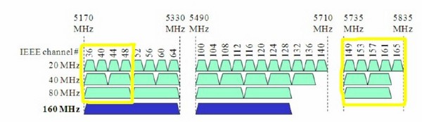
802.11ac Gigabit Wi-Fi spec supports larger channels at 40, 80, and 160 MHz channel

widths instead of 20 MHz widths. This yields increased peak performance and bandwidth

for wireless clients. Planning of channel assignment and widths on 11ac devices requires

a channel plan prior to a WLAN deployment. The full discussion of 802.11ac is beyond

the scope of this article, but a basic discussion for the newest standard 802.11azis presented

at the beginning of this article in an Addendum because the future of Wi-Fi lies within this advanced

technology.

Radio Frequency (RF) Power

 

A typical radio system will consist of a transmitter with a transmitting antenna

sending radio waves through some media to a receiving antenna connected to a

receiver. The radio system transmits information (data packets within a radio

frequency modulation scheme) to the transmitter. The RF signal containing the

data packets is transmitted through an antenna which converts the signal into

an electromagnetic wave. The transmission medium through which the electromagnetic

wave propagates is free space. The electromagnetic wave is intercepted by the

receiving antenna which converts it back to an RF signal that is the same as

the transmitted RF signal. The received RF signal is then demodulated by the

receiver to yield the original information.

 

Because of the wide range of power levels in RF signals, the measurement of

power is expressed in decibels (dB) rather than the Watt as the electrical unit

of power. For analyzing a radio system, the dBm convention is more convenient

than the Watts convention. The RF power level can be expressed in dBm (the subscript

“m” meaning the power is expressed in milliwatts) using the relation between dBm and

Watts as follows:       

 

P dBm = 10 x Log P mw

 

where P dBm = power in decibels

 

P mw = power in milliwatts

 

Some examples are: 1 Watt = 1000 mW;    P dBm = 10 x Log 1000 = 30 dBm

 

                                                500 mW;    P dBm = 10 x Log 500   = 27 dBm

 

                                                100 mW;    P dBm = 10 x Log 100  = 20 dBm

 

                                                  50 mW;    P dBm = 10 x Log 50   = 17 dBm

 

                                                  30 mW;    P dBm = 10 x Log 30   = 14.8 dBm

 

                                                  15 mW;    P dBm = 10 x Log 15   = 11.8 dBm

 

Please note that whenever the power is halved that the dBm value decreases

by 3 dBm. This type of number is a logarithm, which is the exponent expressing

the power to which a fixed base number must be raised to produce a given number.

We are using a base of 10 for our logarithms.

 

Note: Refer to a Logarithm Table.

 

Signal Attenuation

 

An RF signal will fade (decrease in or lose power) as it propagates through

a medium or media. The media could consist of two layers of sheetrock plus

fiberglass insulation and wood framing plus air (a gas) through which an RF signal

propagates, going from one antenna to another. This attenuation (fading) is

expressed in decibels which can be converted to milliwatts. The units of power only need

be expressed in the same units (watts or milliwatts) in the relation

 

P dB = -10 x Log (P out / P in )

 

where P in = the incident power level at the input of the attenuating media

 

           P out = the output power level at the output of the attenuating media

 

           P dB = the attenuation loss expressed in decibels (dB)

 

A diagram for attenuation is shown below.

 

 

Fig. 2 Signal Attenuation

 

For example: If half the power is lost due to attenuation P out= ½ P in), the attenuation in

dB is -10 x Log (½) = -3 dB.

 

Path Loss

 

The Path Loss is the power loss of an RF signal traveling (propagating) through

space or obstructions. It is expressed in dB and depends upon:

The distance between the transmitting and receiving antennas.

The Line of Sight clearance distance between the receiving and transmitting

antennas.

The height of the antenna.

The loss in passing through walls or objects between antennas.

 

 

 

Fig. 3 Path Loss

 

Using the loss value for a sheetrock wall (listed in Table 3 presented later in this

lesson) the path loss would be:

 

Path Loss = Pl = 5 dB

 

 

We will use the path losses in the analysis of received RF signal strength in following

sections of this lesson. Different materials and combinations of materials have different

loss values which can be added directly using decibels to evaluate losses.

 

Free Space Loss

 

The Free Space Loss is an attenuation of the electromagnetic wave while propagating

through space. We will consider the loss to be the same in air as in the vacuum

of space. It is calculated using the following formula:

 

                                    Free Space Loss = 32.4 + 20 x Log F MHz + 20 x Log R Km

where F MHz = the RF frequency expressed in MHz = 2,400 MHz for 802.11b systems

           R Km = the distance in Kilometers between the transmitting and receiving antennas.

 

The formula at 2.4 GHz is: 

Free Space Loss = 100 + 20 x Log R Km

In the following figure, The distance (D) can be expressed in kilometers or

miles, as we will discuss later in this section and consider the conversion

factors between kilometers and miles.

 

 

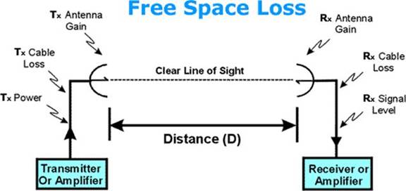
Fig. 4 Free Space Loss

 

The Free Space Loss is not usually a factor in the home and office wireless

network, but can be a factor in linking separate buildings, and definitely should

be included in a discussion of wireless link parameters. To calculate the loss

in units of miles and megahertz, the equation becomes:

Free Space Loss = 36.6 + 20Log 10(Frequency in MHz) + 20Log 10(Distance in Miles)

 

Antenna Characteristics

 

Isotropic Antenna

An Isotropic Antenna is an idealized, theoretical antenna having equal radiation

intensity in all directions. The Isotropic Antenna is used as a zero dB gain

reference in antenna gain (directivity) calculation.

 

Antenna Gain

The Antenna Gain is actually a measure of directivity and is defined as the

ratio of the radiation intensity (power) in a given direction to the radiation

intensity that would be obtained in the same direction from an Isotropic Antenna.

Antenna Gain is expressed in dBi (in other words, it is referenced to an isotropic

radiator). Some of the considerations in placing (mounting) antennas include

down-tilt angle (if any), beamwidth and aiming, and polarization. Most home

and office antenna mountings align the antenna with no down-tilt, especially

if it is an omni-directional antenna. Directional antennas may be mounted with

down or up-tilts depending upon the area of coverage desired in a high or multi-floor

level building. A diagram illustrating antenna tilt geometry follows.

 

 

 

Fig. 5 Antenna Tilt Angle Definition

 

 

The antenna in the above diagram has an axis that aligns with the electric

field vector of the RF signal, which is usually set in a vertical plane (aligns

with gravity vector at any point on the planet). In some point-to-point wireless

network designs, pairs of antennas may be rotated 90 degrees so that the electric

field variation is in the horizontal plane. The plane in which the electric

field variation (vector) aligns is known as the plane of polarization.

So the antenna polarization can be vertical or horizontal. If multiple wireless

networks are operating near one another, even on separate channels, interference

can sometimes be eliminated by changing the polarity of one set of network antennas.

Signal interference from many sources (including 2.4 GHz microwave ovens) can

sometimes be eliminated by a change in antenna polarization, as well as physical

location.

 

Another consideration in down-tilt antenna mounting is reflecting off surfaces

that the main lobe contacts. In a home or office with walls, ceilings, and floors

to bounce (reflect) the RF signal, aiming is important. Try to minimize the

reflections by keeping the angle of incidence as perpendicular (normal) to surfaces

as possible. Low angles of incidence cause more trouble than normal incidence

for RF signals.

 

These considerations are very important when designing outdoor RF signal links

where distances of  miles between antennas exist. Even in modest home and office

link distances, these geometries should be considered. The following diagram

presents a tilted antenna configuration.

 

Fig. 6 Antenna Aiming

 

 

Radiation Pattern

A Radiation Pattern is the spatial energy distribution of an antenna. The spatial

distribution can be shown in rectangular or polar coordinates. The spatial distribution

of a practical antenna exhibits main lobes or lobe, and side lobes. The antenna

manufacturer will specify the radiation pattern for an antenna. The following

illustration shows the main lobe containing most of the RF signal power (energy),

and side lobes containing less RF signal power. The RF signal power radiates

outward from the antenna in all the lobes. This spreads the energy in the RF

signal ever wider which means that a receiving antenna farther away from the

transmitting antenna will receive a lower RF signal power level than a closer

located receiving antenna.

 

 

Fig. 7 Antenna Pattern

 

 

Side Lobes

Radiation lobes in directions other than that of a main lobe(s) are known as

Side Lobes. The antenna manufacturer will specify the radiation pattern

for an antenna. See the previous illustration. Side lobes can transmit enough

RF signal power to allow connection between other antennas.

 

Omnidirectional Antenna

 

An Omnidirectional Antenna radiates and receives equally in all directions

within a “pancake” shaped volume (spatial distribution). The antenna manufacturer

will specify the radiation pattern for an antenna. See the following illustration.</p>

 

 

Fig. 8 Omni Antenna

 

 

Directional Antenna

The radiation pattern of a Directional Antenna is predominantly in one direction.

The antenna still has side lobes, but the main lobe contains most of the radiated

and received power.  The antenna manufacturer will specify the radiation pattern

for an antenna. Refer to the previous Antenna Radiation Power diagram as an

example of a directional antenna radiation pattern.

 

Antenna Beamwidth

The Antenna Beamwidth is defined as the RF Power included angle of a directional

antenna. The definition is the angle between two half-power (-3 dB) points on

either side of the main radiation lobe. The antenna manufacturer will specify the radiation

pattern for an antenna.  Refer to the previous illustrations.

 

System Characteristics

 

Receiver Sensitivity (Ps)

The receiver sensitivity is the minimum RF signal power level required at the

input of the receiver for satisfactory system performance. This parameter is

usually specified by the radio equipment manufacturer. <b>Ps</b> in dBm is the

receiver sensitivity.

Effective Isotropic Radiated Power (EIRP)

The EIRP is the antenna transmitted power, which equals the RF signal output

power minus antenna cable loss plus the transmitting antenna gain. The equation

is:

 

        EIRP = P out – Ct + Gt

 

where P out = transmitted output RF power to antenna in dBm

            Ct = transmitter cable attenuation in dB

            Gt = transmitting antenna gain in dBi

 

Effective Received RF Signal Power (Si)

 

The effective received signal power can be calculated using the following equation:

 

                                    Si = EIRP – Pl + Gr –Cr = P out – Ct + Gt – Pl + Gr – Cr

 

Where Pl = Path loss in dB

            Gr = receiving antenna gain in dBi

            Cr = receiver cable attenuation in dB

 

Example:  Wireless System Link Analysis

            Frequency = 2.4 GHz

            P out = 4 dBm (2.5 mW)

Tx and Rx cable loss for 10 meter cable type RG214 (0.6 dB/meter)

            Ct = Cr = 6 dB

Tx and Rx antenna gain

            Gt = Gr = 18 dBi

Distance between antennas R Km = 3 Km

            Pl = 100 + 20 x Log(R Km) = 110 dB

Receiver sensitivity  Ps = -84 dBm

Calculate:

EIRP = P out – Ct + Gt = 16 dBm

Si = EIRP + Gr – Cr = 16 – (110) = -82 dBm

 

Analysis of the above result: The received signal power (Si) is above the sensitivity

threshold of the receiver (Ps), so the link should work. However, Si should

be at least 10 dB higher than Ps. In this case, the signal is only 2 dB higher

and we really should consider another loss factor, Signal Fading. A better system

solution would be to increase the transmit RF signal power to P out = 10 dBm, which is a

power of 10 milliwatts.

 

Signal Fading

RF signal fading is caused by several factors including: Multipath Reception,

Line of Sight Interference, Fresnel Zone Interference, RF Interference, Weather

Conditions.

Multipath Reception – The transmitted signal arrives at the receiver

from different directions, with different path lengths, attenuation, and delays.

An RF reflective surface, like a cement surface or roof surfaces, can yield

multiple paths between antennas. The higher the antenna mount position is from

such surfaces, the lower the multiple path losses. The radio equipment in the

802.11 specifications utilizes modulation schemes and reception methods such

that multiple path problems are minimized.

 

Line of Sight Interference– A clear, straight line of sight between

the system antennas is absolutely required for a proper RF link for long distances

outdoors. A clear line of sight exists if an unobstructed view of one antenna

from the other antenna. A radio wave clear line of sight exists if a defined

area around the optical line of sight is also clear of obstacles. Remember that

the electric and magnetic fields are perpendicular to the direction of propagation

of the RF wave. In setting up wireless networks in buildings, propagation of

the RF signal through walls and other items is a fact of life. If you recall

the signal attenuation discussion earlier, we can evaluate the related losses.

A following table presents loss values for typical items through which we want

our networks to transmit and receive.

Fresnel Zone Interference – The Fresnel (FRA-nel) Zone is a circular

area perpendicular to and centered on the line of sight. In radio wave theory,

if 80% of the first Fresnel Zone is clear of obstacles, the wave propagation

loss is equivalent to that of free space.

 

 

Fig. 9 Fresnel Zone

 

 

The equation for calculating the first Fresnel Zone utilizes distances to a

point in the line of sight with a possible obstruction in the path is:

                        FZ =  72.1 x sq. root (D1 x D2) / (f  x R m )

where   f = frequency in GHz

                        R m = distance between antennas in miles

                        D1  =  first distance to obstruction in miles

                        D2  =  second distance to obstruction in miles = R m – D1

                        FZ  =  radius of Fresnel Zone in feet from direct line of sight

 

We will calculate a Fresnel Zone radius later in this discussion.  In the home

and office network in a building, the Fresnel Zone calculation is usually unnecessary

because of all the wall/ceiling/floor pass- through considerations for any RF

signal path. But in outside RF signal paths (links), the Fresnel Zone calculations

can be very important from quarter mile distances and longer.

My experience with tall loblolly pines on a project is a good case in point.

A wireless link was designed and setup for two medical facilities (two-story

structures) in Wilmington, NC which were located 0.5 and 0.75 miles from an eleven-

story hospital. There was no direct line of sight between the two medical facilities, but

there was from both buildings to the hospital roof. After securing proper approvals, an RF

signal link was setup from each building antenna to hospital roof-mounted antennas.

Even though there was a good visual path from one building to the hospital roof,

some very tall, very scrawny loblolly pines were infringing into the Fresnel

Zone radius that was calculated for the link. It was just a few branches with

the wide-spaced loblolly needles, but we had to top the trees to obtain a satisfactory

signal-to-noise ratio for dependable communication. It is amazing how much

microwave (2.4 GHz) energy those long needles absorbed, reflected, deflected, and/or

scattered.

 

In the earlier wireless link analysis example using the 3 Km distance between

antennas and assuming a mid-path constriction (D1 = D2), the Fresnel Zone is

calculated as follows using common conversion factors for US standard measurements.

               

Convert 3 Km to miles by dividing by a conversion factor of 1.6 kilometers per mile,

which yields using f = 2.4 GHz:

R m = 3Km / 1.6Km/mile = 1.88 miles

D1 = D2 = 0.94 mile

FZ = 31.9 feet

The 80% Fresnel Zone radius for Free Space Loss equivalence would be obtained

by multiplying FZ by 0.8, which yields a radius of 25.5 feet. So the clear path

concentric cylinder around your systems line of sight for the distances and

frequency analyzed would be 51 feet in diameter at the middle of the RF link.

 

System Operating Margin (SOM)

SOM (System Operating Margin), also known as fade

margin, is the difference of the receiver signal level in dBm minus the receiver

sensitivity in dBm. It is a measure of the safety margin in a radio link. A

higher SOM means a more reliable over the air connection. We recommend a minimum

of 10 dB, but 20 dB or more is better for reliable, high bandwidth connections.

 

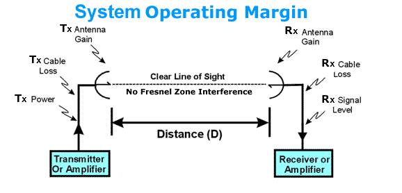
Fig. 10 Signal Operating Margin

 

SOM is the difference between the signal a radio is actually receiving vs. what it needs

for good data recovery (i.e. receiver sensitivity). By using the transmit and receive RF

signal power, the cable losses, the antenna gains, and the free space losses as considered

in this lesson, we can calculate the SOM. Thus we have a method for designing and

analyzing RF signal links used in wireless networking.

 

Rx Signal Level = Tx Power - Tx Cable Loss + Tx Antenna Gain – Free Space Loss + Rx Antenna Gain - Rx Cable Loss

SOM = Rx Signal Level - Rx Sensitivity

We can modify the SOM expression to consider attenuation losses due to transmission

through walls, etc., in an actual building wherein a home or office network would be

installed. It is simply adding more loss terms to the SOM equation. But first we will have

to consider the level of losses through various materials. The signal attenuation loss for

2.4 GHz transmission through the following structures can be included in the Rx Signal

Level equation for each pass-through in the straight line signal path (line of sight). The

dB loss values will be subtracted from the transmitted signal power to reflect the loss of

passing through the material structures.

 

Structure	Loss, dB
Clear Glass Window	2
Brick Wall	2
Brick Wall next to a Metal Door	3
Cinder Block Wall	4
Sheetrock/Wood Frame Wall	5
Sheetrock/Metal Framed Wall	6
Metal Frame Clear Glass Wall	6
Metal Screened Clear Glass Window	6
Metal Door in Office Wall	6
Wired-Glass Window	8
Metal Door in Brick Wall	12

Table 3 Transmission Losses

 

The loss for each structure passed through should be included in the calculations of Rx

Signal Level and SOM. The minimum SOM suggested is 15 dB, but a 25 dB margin

should be used in all designs as the real world losses are almost always higher than the

theoretical. The loss factors for walls or objects can be measured by using a wireless

signal source (router, access point, etc.) with output measured before and after the object.

 

Conclusion

Using the contents of this lesson any wireless network can be designed or analyzed.

All of the content of this article was presented to lead up to the ability to

understand and apply all the factors that comprise a wireless network's Effective

Received RF Signal Power (Si) and the System Operating Margin (SOM).

These two parameters are central to the design, analysis, and performance of any wireless

network.

 

That said, most Wi-Fi systems are not formally designed with Si or SOM analyses, but

rather Wi-Fi components are selected from available products in a price range of interest.

An on-site wireless survey using wireless devices including any intended antennas and a

laptop, tablet, or smartphone with an app to read signal power levels can be setup around

the site and signal tested. The system is then configured, installed and tested. Sometimes

it works satisfactorily and sometimes not. If not, the above radio physics topics can be

utilized to analyze the problem and then fix it. Good and bad signal level measurements

can be utilized to add access points, repeaters, higher gain antennas, etc., to obtain

reliable area coverage.